3 Competency 3
Chapter 4. Hypothesis Testing
Hypothesis testing is the other widely used form of inferential statistics. It is different from estimation because you start a hypothesis test with some idea of what the population is like and then test to see if the sample supports your idea. Though the mathematics of hypothesis testing is very much like the mathematics used in interval estimation, the inference being made is quite different. In estimation, you are answering the question, “What is the population like?” While in hypothesis testing you are answering the question, “Is the population like this or not?”
A hypothesis is essentially an idea about the population that you think might be true, but which you cannot prove to be true. While you usually have good reasons to think it is true, and you often hope that it is true, you need to show that the sample data support your idea. Hypothesis testing allows you to find out, in a formal manner, if the sample supports your idea about the population. Because the samples drawn from any population vary, you can never be positive of your finding, but by following generally accepted hypothesis testing procedures, you can limit the uncertainty of your results.
As you will learn in this chapter, you need to choose between two statements about the population. These two statements are the hypotheses. The first, known as the null hypothesis, is basically, “The population is like this.” It states, in formal terms, that the population is no different than usual. The second, known as the alternative hypothesis, is, “The population is like something else.” It states that the population is different than the usual, that something has happened to this population, and as a result it has a different mean, or different shape than the usual case. Between the two hypotheses, all possibilities must be covered. Remember that you are making an inference about a population from a sample. Keeping this inference in mind, you can informally translate the two hypotheses into “I am almost positive that the sample came from a population like this” and “I really doubt that the sample came from a population like this, so it probably came from a population that is like something else”. Notice that you are never entirely sure, even after you have chosen the hypothesis, which is best. Though the formal hypotheses are written as though you will choose with certainty between the one that is true and the one that is false, the informal translations of the hypotheses, with “almost positive” or “probably came”, is a better reflection of what you actually find.
Hypothesis testing has many applications in business, though few managers are aware that that is what they are doing. As you will see, hypothesis testing, though disguised, is used in quality control, marketing, and other business applications. Many decisions are made by thinking as though a hypothesis is being tested, even though the manager is not aware of it. Learning the formal details of hypothesis testing will help you make better decisions and better understand the decisions made by others.
The next section will give an overview of the hypothesis testing method by following along with a young decision-maker as he uses hypothesis testing. Additionally, with the provided interactive Excel template, you will learn how the results of the examples from this chapter can be adjusted for other circumstances. The final section will extend the concept of hypothesis testing to categorical data, where we test to see if two categorical variables are independent of each other. The rest of the chapter will present some specific applications of hypothesis tests as examples of the general method.
The strategy of hypothesis testing
Usually, when you use hypothesis testing, you have an idea that the world is a little bit surprising; that it is not exactly as conventional wisdom says it is. Occasionally, when you use hypothesis testing, you are hoping to confirm that the world is not surprising, that it is like conventional wisdom predicts. Keep in mind that in either case you are asking, “Is the world different from the usual, is it surprising?” Because the world is usually not surprising and because in statistics you are never 100 per cent sure about what a sample tells you about a population, you cannot say that your sample implies that the world is surprising unless you are almost positive that it does. The dull, unsurprising, usual case not only wins if there is a tie, it gets a big lead at the start. You cannot say that the world is surprising, that the population is unusual, unless the evidence is very strong. This means that when you arrange your tests, you have to do it in a manner that makes it difficult for the unusual, surprising world to win support.
The first step in the basic method of hypothesis testing is to decide what value some measure of the population would take if the world was unsurprising. Second, decide what the sampling distribution of some sample statistic would look like if the population measure had that unsurprising value. Third, compute that statistic from your sample and see if it could easily have come from the sampling distribution of that statistic if the population was unsurprising. Fourth, decide if the population your sample came from is surprising because your sample statistic could not easily have come from the sampling distribution generated from the unsurprising population.
That all sounds complicated, but it is really pretty simple. You have a sample and the mean, or some other statistic, from that sample. With conventional wisdom, the null hypothesis that the world is dull, and not surprising, tells you that your sample comes from a certain population. Combining the null hypothesis with what statisticians know tells you what sampling distribution your sample statistic comes from if the null hypothesis is true. If you are almost positive that the sample statistic came from that sampling distribution, the sample supports the null. If the sample statistic “probably came” from a sampling distribution generated by some other population, the sample supports the alternative hypothesis that the population is “like something else”.
Imagine that Thad Stoykov works in the marketing department of Pedal Pushers, a company that makes clothes for bicycle riders. Pedal Pushers has just completed a big advertising campaign in various bicycle and outdoor magazines, and Thad wants to know if the campaign has raised the recognition of the Pedal Pushers brand so that more than 30 per cent of the potential customers recognize it. One way to do this would be to take a sample of prospective customers and see if at least 30 per cent of those in the sample recognize the Pedal Pushers brand. However, what if the sample is small and just barely 30 per cent of the sample recognizes Pedal Pushers? Because there is variance among samples, such a sample could easily have come from a population in which less than 30 per cent recognize the brand. If the population actually had slightly less than 30 per cent recognition, the sampling distribution would include quite a few samples with sample proportions a little above 30 per cent, especially if the samples are small. In order to be comfortable that more than 30 per cent of the population recognizes Pedal Pushers, Thad will want to find that a bit more than 30 per cent of the sample does. How much more depends on the size of the sample, the variance within the sample, and how much chance he wants to take that he’ll conclude that the campaign did not work when it actually did.
Let us follow the formal hypothesis testing strategy along with Thad. First, he must explicitly describe the population his sample could come from in two different cases. The first case is the unsurprising case, the case where there is no difference between the population his sample came from and most other populations. This is the case where the ad campaign did not really make a difference, and it generates the null hypothesis. The second case is the surprising case when his sample comes from a population that is different from most others. This is where the ad campaign worked, and it generates the alternative hypothesis. The descriptions of these cases are written in a formal manner. The null hypothesis is usually called Ho. The alternative hypothesis is called either H1 or Ha. For Thad and the Pedal Pushers marketing department, the null hypothesis will be:
Ho: proportion of the population recognizing Pedal Pushers brand < .30
and the alternative will be:
Ha: proportion of the population recognizing Pedal Pushers brand >.30
Notice that Thad has stacked the deck against the campaign having worked by putting the value of the population proportion that means that the campaign was successful in the alternative hypothesis. Also notice that between Ho and Ha all possible values of the population proportion (>, =, and < .30) have been covered.
Second, Thad must create a rule for deciding between the two hypotheses. He must decide what statistic to compute from his sample and what sampling distribution that statistic would come from if the null hypothesis, Ho, is true. He also needs to divide the possible values of that statistic into usual and unusual ranges if the null is true. Thad’s decision rule will be that if his sample statistic has a usual value, one that could easily occur if Ho is true, then his sample could easily have come from a population like that which described Ho. If his sample’s statistic has a value that would be unusual if Ho is true, then the sample probably comes from a population like that described in Ha. Notice that the hypotheses and the inference are about the original population while the decision rule is about a sample statistic. The link between the population and the sample is the sampling distribution. Knowing the relative frequency of a sample statistic when the original population has a proportion with a known value is what allows Thad to decide what are usual and unusual values for the sample statistic.
The basic idea behind the decision rule is to decide, with the help of what statisticians know about sampling distributions, how far from the null hypothesis’ value for the population the sample value can be before you are uncomfortable deciding that the sample comes from a population like that hypothesized in the null. Though the hypotheses are written in terms of descriptive statistics about the population—means, proportions, or even a distribution of values—the decision rule is usually written in terms of one of the standardized sampling distributions—the t, the normal z, or another of the statistics whose distributions are in the tables at the back of statistics textbooks. It is the sampling distributions in these tables that are the link between the sample statistic and the population in the null hypothesis. If you learn to look at how the sample statistic is computed you will see that all of the different hypothesis tests are simply variations on a theme. If you insist on simply trying to memorize how each of the many different statistics is computed, you will not see that all of the hypothesis tests are conducted in a similar manner, and you will have to learn many different things rather than the variations of one thing.
Thad has taken enough statistics to know that the sampling distribution of sample proportions is normally distributed with a mean equal to the population proportion and a standard deviation that depends on the population proportion and the sample size. Because the distribution of sample proportions is normally distributed, he can look at the bottom line of a t-table and find out that only .05 of all samples will have a proportion more than 1.645 standard deviations above .30 if the null hypothesis is true. Thad decides that he is willing to take a 5 per cent chance that he will conclude that the campaign did not work when it actually did. He therefore decides to conclude that the sample comes from a population with a proportion greater than .30 that has heard of Pedal Pushers, if the sample’s proportion is more than 1.645 standard deviations above .30. After doing a little arithmetic (which you’ll learn how to do later in the chapter), Thad finds that his decision rule is to decide that the campaign was effective if the sample has a proportion greater than .375 that has heard of Pedal Pushers. Otherwise the sample could too easily have come from a population with a proportion equal to or less than .30.
| alpha | .1 | .05 | .03 | .01 |
|---|---|---|---|---|
| df infinity | 1.28 | 1.65 | 1.96 | 2.33 |
The final step is to compute the sample statistic and apply the decision rule. If the sample statistic falls in the usual range, the data support Ho, the world is probably unsurprising, and the campaign did not make any difference. If the sample statistic is outside the usual range, the data support Ha, the world is a little surprising, and the campaign affected how many people have heard of Pedal Pushers. When Thad finally looks at the sample data, he finds that .39 of the sample had heard of Pedal Pushers. The ad campaign was successful!
A straightforward example: testing for goodness-of-fit
There are many different types of hypothesis tests, including many that are used more often than the goodness-of-fit test. This test will be used to help introduce hypothesis testing because it gives a clear illustration of how the strategy of hypothesis testing is put to use, not because it is used frequently. Follow this example carefully, concentrating on matching the steps described in previous sections with the steps described in this section. The arithmetic is not that important right now.
We will go back to Chapter 1, where the Chargers’ equipment manager, Ann, at Camosun College, collected some data on the size of the Chargers players’ sport socks. Recall that she asked both the basketball and volleyball team managers to collect these data, shown in Table 4.2.
David, the marketing manager of the company that produces these socks, contacted Ann to tell her that he is planning to send out some samples to convince the Chargers players that wearing Easy Bounce socks will be more comfortable than wearing other socks. He needs to include an assortment of sizes in those packages and is trying to find out what sizes to include. The Production Department knows what mix of sizes they currently produce, and Ann has collected a sample of 97 basketball and volleyball players’ sock sizes. David needs to test to see if his sample supports the hypothesis that the collected sample from Camosun college players has the same distribution of sock sizes as the company is currently producing. In other words, is the distribution of Chargers players’ sock sizes a good fit to the distribution of sizes now being produced (see Table 4.2)?
| Size | Frequency | Relative Frequency |
|---|---|---|
| 6 | 3 | .031 |
| 7 | 24 | .247 |
| 8 | 33 | .340 |
| 9 | 20 | .206 |
| 10 | 17 | .175 |
From the Production Department, the current relative frequency distribution of Easy Bounce socks in production is shown in Table 4.3.
| Size | Relative Frequency |
|---|---|
| 6 | .06 |
| 7 | .13 |
| 8 | .22 |
| 9 | .3 |
| 10 | .26 |
| 11 | .03 |
If the world is unsurprising, the players will wear the socks sized in the same proportions as other athletes, so David writes his hypotheses:
Ho: Chargers players’ sock sizes are distributed just like current production.
Ha: Chargers players’ sock sizes are distributed differently.
Ann’s sample has n=97. By applying the relative frequencies in the current production mix, David can find out how many players would be expected to wear each size if the sample was perfectly representative of the distribution of sizes in current production. This would give him a description of what a sample from the population in the null hypothesis would be like. It would show what a sample that had a very good fit with the distribution of sizes in the population currently being produced would look like.
Statisticians know the sampling distribution of a statistic that compares the expected frequency of a sample with the actual, or observed, frequency. For a sample with c different classes (the sizes here), this statistic is distributed like χ2 with c-1 df. The χ2 is computed by the formula:
[latex]sample\;chi^2 = \sum{((O-E)^2)/E}[/latex]
where
O = observed frequency in the sample in this class
E = expected frequency in the sample in this class
The expected frequency, E, is found by multiplying the relative frequency of this class in the Ho hypothesized population by the sample size. This gives you the number in that class in the sample if the relative frequency distribution across the classes in the sample exactly matches the distribution in the population.
Notice that χ2 is always > 0 and equals 0 only if the observed is equal to the expected in each class. Look at the equation and make sure that you see that a larger value of χ2 goes with samples with large differences between the observed and expected frequencies.
David now needs to come up with a rule to decide if the data support Ho or Ha. He looks at the table and sees that for 5 df (there are 6 classes—there is an expected frequency for size 11 socks), only .05 of samples drawn from a given population will have a χ2 > 11.07 and only .10 will have a χ2 > 9.24. He decides that it would not be all that surprising if the players had a different distribution of sock sizes than the athletes who are currently buying Easy Bounce, since all of the players are women and many of the current customers are men. As a result, he uses the smaller .10 value of 9.24 for his decision rule. Now David must compute his sample χ2. He starts by finding the expected frequency of size 6 socks by multiplying the relative frequency of size 6 in the population being produced by 97, the sample size. He gets E = .06*97=5.82. He then finds O-E = 3-5.82 = -2.82, squares that, and divides by 5.82, eventually getting 1.37. He then realizes that he will have to do the same computation for the other five sizes, and quickly decides that a spreadsheet will make this much easier (see Table 4.4).
| Sock Size | Frequency in Sample | Population Relative Frequency | Expected Frequency = 97*C | (O-E)^2/E |
|---|---|---|---|---|
| 6 | 3 | .06 | 5.82 | 1.3663918 |
| 7 | 24 | .13 | 12.61 | 10.288033 |
| 8 | 33 | .22 | 21.34 | 6.3709278 |
| 9 | 20 | .3 | 29.1 | 2.8457045 |
| 10 | 17 | .26 | 25.22 | 2.6791594 |
| 11 | 0 | .03 | 2.91 | 2.91 |
| 97 | χ2 = 26.460217 |
David performs his third step, computing his sample statistic, using the spreadsheet. As you can see, his sample χ2 = 26.46, which is well into the unusual range that starts at 9.24 according to his decision rule. David has found that his sample data support the hypothesis that the distribution of sock sizes of the players is different from the distribution of sock sizes that are currently being manufactured. If David’s employer is going to market Easy Bounce socks to the BC college players, it is going to have to send out packages of samples that contain a different mix of sizes than it is currently making. If Easy Bounce socks are successfully marketed to the BC college players, the mix of sizes manufactured will have to be altered.
Now review what David has done to test to see if the data in his sample support the hypothesis that the world is unsurprising and that the players have the same distribution of sock sizes as the manufacturer is currently producing for other athletes. The essence of David’s test was to see if his sample χ2 could easily have come from the sampling distribution of χ2’s generated by taking samples from the population of socks currently being produced. Since his sample χ2 would be way out in the tail of that sampling distribution, he judged that his sample data supported the other hypothesis, that there is a difference between the Chargers players and the athletes who are currently buying Easy Bounce socks.
Formally, David first wrote null and alternative hypotheses, describing the population his sample comes from in two different cases. The first case is the null hypothesis; this occurs if the players wear socks of the same sizes in the same proportions as the company is currently producing. The second case is the alternative hypothesis; this occurs if the players wear different sizes. After he wrote his hypotheses, he found that there was a sampling distribution that statisticians knew about that would help him choose between them. This is the χ2 distribution. Looking at the formula for computing χ2 and consulting the tables, David decided that a sample χ2 value greater than 9.24 would be unusual if his null hypothesis was true. Finally, he computed his sample statistic and found that his χ2, at 26.46, was well above his cut-off value. David had found that the data in his sample supported the alternative χ2: that the distribution of the players’ sock sizes is different from the distribution that the company is currently manufacturing. Acting on this finding, David will include a different mix of sizes in the sample packages he sends to team coaches.
Testing population proportions
As you learned in Chapter 3, sample proportions can be used to compute a statistic that has a known sampling distribution. Reviewing, the z-statistic is:
[latex]z = (p-\pi)/\sqrt{\dfrac{(\pi)(1-\pi)}{n}}[/latex]
where
p = the proportion of the sample with a certain characteristic
π = the proportion of the population with that characteristic
[latex]\sqrt{\dfrac{(\pi)(1-\pi)}{n}}[/latex] = the standard deviation (error) of the proportion of the population with that characteristic
As long as the two technical conditions of π*n and (1-π)*n are held, these sample z-statistics are distributed normally so that by using the bottom line of the t-table, you can find what portion of all samples from a population with a given population proportion, π, have z-statistics within different ranges. If you look at the z-table, you can see that .95 of all samples from any population have z-statistics between ±1.96, for instance.
If you have a sample that you think is from a population containing a certain proportion, π, of members with some characteristic, you can test to see if the data in your sample support what you think. The basic strategy is the same as that explained earlier in this chapter and followed in the goodness-of-fit example: (a) write two hypotheses, (b) find a sample statistic and sampling distribution that will let you develop a decision rule for choosing between the two hypotheses, and (c) compute your sample statistic and choose the hypothesis supported by the data.
Foothill Hosiery recently received an order for children’s socks decorated with embroidered patches of cartoon characters. Foothill did not have the right machinery to sew on the embroidered patches and contracted out the sewing. While the order was filled and Foothill made a profit on it, the sewing contractor’s price seemed high, and Foothill had to keep pressure on the contractor to deliver the socks by the date agreed upon. Foothill’s CEO, John McGrath, has explored buying the machinery necessary to allow Foothill to sew patches on socks themselves. He has discovered that if more than a quarter of the children’s socks they make are ordered with patches, the machinery will be a sound investment. John asks Kevin to find out if more than 35 per cent of children’s socks are being sold with patches.
Kevin calls the major trade organizations for the hosiery, embroidery, and children’s clothes industries, and no one can answer his question. Kevin decides it must be time to take a sample and test to see if more than 35 per cent of children’s socks are decorated with patches. He calls the sales manager at Foothill, and she agrees to ask her salespeople to look at store displays of children’s socks, counting how many pairs are displayed and how many of those are decorated with patches. Two weeks later, Kevin gets a memo from the sales manager, telling him that of the 2,483 pairs of children’s socks on display at stores where the salespeople counted, 826 pairs had embroidered patches.
Kevin writes his hypotheses, remembering that Foothill will be making a decision about spending a fair amount of money based on what he finds. To be more certain that he is right if he recommends that the money be spent, Kevin writes his hypotheses so that the unusual world would be the one where more than 35 per cent of children’s socks are decorated:
Ho: π decorated socks < .35
Ha: π decorated socks > .35
When writing his hypotheses, Kevin knows that if his sample has a proportion of decorated socks well below .35, he will want to recommend against buying the machinery. He only wants to say the data support the alternative if the sample proportion is well above .35. To include the low values in the null hypothesis and only the high values in the alternative, he uses a one-tail test, judging that the data support the alternative only if his z-score is in the upper tail. He will conclude that the machinery should be bought only if his z-statistic is too large to have easily come from the sampling distribution drawn from a population with a proportion of .35. Kevin will accept Ha only if his z is large and positive.
Checking the bottom line of the t-table, Kevin sees that .95 of all z-scores associated with the proportion are less than -1.645. His rule is therefore to conclude that his sample data support the null hypothesis that 35 per cent or less of children’s socks are decorated if his sample (calculated) z is less than -1.645. If his sample z is greater than -1.645, he will conclude that more than 35 per cent of children’s socks are decorated and that Foothill Hosiery should invest in the machinery needed to sew embroidered patches on socks.
Using the data the salespeople collected, Kevin finds the proportion of the sample that is decorated:
[latex]\pi = 826/2483 = .333[/latex]
Using this value, he computes his sample z-statistic:
[latex]z = (p-\pi)/(\sqrt{\dfrac{(\pi)(1-\pi)}{n}}) = (.333-.35)/(\sqrt{\dfrac{(.35)(1-.35)}{2483}}) = \dfrac{-.0173}{.0096} = -1.0811[/latex]
All these calculations, along with the plots of both sampling distribution of π and the associated standard normal distributions, are computed by the interactive Excel template in Figure 4.1.
Figure 4.1 Interactive Excel Template for Test of Hypothesis – see Appendix 4.
Kevin’s collected numbers, shown in the yellow cells of Figure 4.1., can be changed to other numbers of your choice to see how the business decision may be changed under alternative circumstances.
Because his sample (calculated) z-score is larger than -1.645, it is unlikely that his sample z came from the sampling distribution of z’s drawn from a population where π < .35, so it is unlikely that his sample comes from a population with π < .35. Kevin can tell John McGrath that the sample the salespeople collected supports the conclusion that more than 35 per cent of children’s socks are decorated with embroidered patches. John can feel comfortable making the decision to buy the embroidery and sewing machinery.
Testing independence and categorical variables
We also use hypothesis testing when we deal with categorical variables. Categorical variables are associated with categorical data. For instance, gender is a categorical variable as it can be classified into two or more categories. In business, and predominantly in marketing, we want to determine on which factor(s) customers base their preference for one type of product over others. Since customers’ preferences are not the same even in a specific geographical area, marketing strategists and managers are often keen to know the association among those variables that affect shoppers’ choices. In other words, they want to know whether customers’ decisions are statistically independent of a hypothesized factor such as age.
For example, imagine that the owner of a newly established family restaurant in Burnaby, BC, with branches in North Vancouver, Langley, and Kelowna, is interested in determining whether the age of the restaurant’s customers affects which dishes they order. If it does, she will explore the idea of charging different prices for dishes popular with different age groups. The sales manager has collected data on 711 sales of different dishes over the last six months, along with the approximate age of the customers, and divided the customers into three categories. Table 4.5 shows the breakdown of orders and age groups.
| Orders | ||||||
| Fish | Veggie | Steak | Spaghetti | Total | ||
| Age Groups | Kids | 26 | 21 | 15 | 20 | 82 |
| Adults | 100 | 74 | 60 | 70 | 304 | |
| Seniors | 90 | 45 | 80 | 110 | 325 | |
| Total | 216 | 140 | 155 | 200 | 711 | |
The owner writes her hypotheses:
Ho: Customers’ preferences for dishes are independent of their ages
Ha: Customers’ preferences for dishes depend on their ages
The underlying test for this contingency table is known as the chi-square test. This will determine if customers’ ages and preferences are independent of each other.
We compute both the observed and expected frequencies as we did in the earlier example involving sports socks where O = observed frequency in the sample in each class, and E = expected frequency in the sample in each class. Then we calculate the expected frequency for the above table with i rows and j columns, using the following formula:
This chi-square distribution will have (i-1)(j-1) degrees of freedom. One technical condition for this test is that the value for each of the cells must not be less than 5. Figure 4.2 provides the hypothesized values for different levels of significance.
The expected frequency, Eij, is found by multiplying the relative frequency of each row and column, and then dividing this amount by the total sample size. Thus,
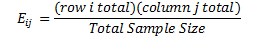
For each of the expected frequencies, we select the associated total row from each of the age groups, and multiply it by the total of the same column, then divide it by the total sample size. For the first row and column, we multiply (82 *216)/711=24.95. Table 4.6 summarizes all expected frequencies for this example.
| Orders | ||||||
|---|---|---|---|---|---|---|
| Fish | Veggie | Steak | Spaghetti | Total | ||
| Age Groups | Kids | 24.95 | 16.15 | 17.88 | 23.07 | 82 |
| Adults | 92.35 | 59.86 | 66.27 | 85.51 | 304 | |
| Seniors | 98.73 | 63.99 | 70.85 | 91.42 | 325 | |
| Total | 216 | 140 | 155 | 200 | 711 | |
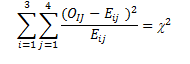
Now we use the calculated expected frequencies and the observed frequencies to compute the chi-square test statistic:
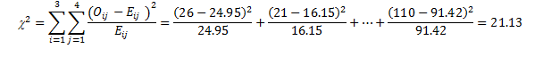
We computed the sample test statistic as 21.13, which is above the 12.592 cut-off value of the chi-square table associated with (3-1)*(4-1) = 6 df at .05 level. To find out the exact cut-off point from the chi-square table, you can enter the alpha level of .05 and the degrees of freedom, 6, directly into the yellow cells in the following interactive Excel template (Figure 4.2). This template contains two sheets; it will plot the chi-square distribution for this example and will automatically show the exact cut-off point.
Figure 4.2 Interactive Excel Template for Determining Chi-Square Cut-off Point – see Appendix 4.
The result indicates that our sample data supported the alternative hypothesis. In other words, customers’ preferences for different dishes depended on their age groups. Based on this outcome, the owner may differentiate price based on these different age groups.
Using the test of independence, the owner may also go further to find out if such dependency exists among any other pairs of categorical data. This time, she may want to collect data for the selected age groups at different locations of her restaurant in British Columbia. The results of this test will reveal more information about the types of customers these restaurants attract at different locations. Depending on the availability of data, such statistical analysis can also be carried out to help determine an improved pricing policy for different groups in different locations, at different times of day, or on different days of the week. Finally, the owner may also redo this analysis by including other characteristics of these customers, such as education, gender, etc., and their choice of dishes.
Summary
This chapter has been an introduction to hypothesis testing. You should be able to see the relationship between the mathematics and strategies of hypothesis testing and the mathematics and strategies of interval estimation. When making an interval estimate, you construct an interval around your sample statistic based on a known sampling distribution. When testing a hypothesis, you construct an interval around a hypothesized population parameter, using a known sampling distribution to determine the width of that interval. You then see if your sample statistic falls within that interval to decide if your sample probably came from a population with that hypothesized population parameter. Hypothesis testing also has implications for decision-making in marketing, as we saw when we extended our discussion to include the test of independence for categorical data.
Hypothesis testing is a widely used statistical technique. It forces you to think ahead about what you might find. By forcing you to think ahead, it often helps with decision-making by forcing you to think about what goes into your decision. All of statistics requires clear thinking, and clear thinking generally makes better decisions. Hypothesis testing requires very clear thinking and often leads to better decision-making.
Chapter 5. The t-Test
In Chapter 3, a sampling distribution, the t-distribution, was introduced. In Chapter 4, you learned how to use the t-distribution to make an important inference, an interval estimate of the population mean. Here you will learn how to use that same t-distribution to make more inferences, this time in the form of hypothesis tests. You will learn how to use the t-test in three different types of hypotheses. You will also have a chance to use the interactive Excel templates to apply the t-test in alternative situations. Before we start to learn about those tests, a quick review of the t-distribution is in order.
The t-distribution
The t-distribution is a sampling distribution. You could generate your own t-distribution with n-1 degrees of freedom by starting with a normal population, choosing all possible samples of one size, n, computing a t-score for each sample, where:
[latex]t = (\bar{x} -\mu)/(s/\sqrt{n})[/latex]
x = the sample mean
μ = the population mean
s = the sample standard deviation
n = the size of the sample
When you have all of the samples’ t-scores, form a relative frequency distribution and you will have your t-distribution. Luckily, you do not have to generate your own t-distributions because any statistics book has a table that shows the shape of the t-distribution for many different degrees of freedom. As introduced in Chapter 2, Figure 5.1 reproduces a portion of a typical t-table within an interactive Excel template.
Figure 5.1 Interactive Excel Template for Determining Cut-off Point of a t-Table – see Appendix 5.
When you look at the formula for the t-score, you should be able to see that the mean t-score is zero because the mean of the x’s is equal to μ. Because most samples have x’s that are close to μ, most will have t-scores that are close to zero. The t-distribution is symmetric, because half of the samples will have x’s greater than μ, and half less. As you can see from the table, if there are 10 df, only .005 of the samples taken from a normal population will have a t-score greater than +3.17. Because the distribution is symmetric, .005 also have a t-score less than -3.17. Ninety-nine per cent of samples will have a t-score between ±3.17. Like the example in Figure 5.1, most t-tables have a picture showing what is in the body of the table. In Figure 5.1, the shaded area is in the right tail, the body of the table shows the t-score that leaves the α in the right tail. This t-table also lists the two-tail α above the one-tail where p = .xx. For 5 df, there is a .05 probability that a sample will have a t-score greater than 2.02, and a .10 probability that a sample will have a t-score either > +2.02 or < -2.02.
There are other sample statistics that follow this same shape and can be used as the basis for different hypothesis tests. You will see the t-distribution used to test three different types of hypotheses in this chapter, and in later chapters, you will see that the t-distribution can be used to test other hypotheses.
Though t-tables show how the sampling distribution of t-scores is shaped if the original population is normal, it turns out that the sampling distribution of t-scores is very close to the one in the table even if the original population is not quite normal, and most researchers do not worry too much about the normality of the original population. An even more important fact is that the sampling distribution of t-scores is very close to the one in the table even if the original population is not very close to being normal as long as the samples are large. This means that you can safely use the t-distribution to make inferences when you are not sure that the population is normal as long as you are sure that it is bell-shaped. You can also make inferences based on samples of about 30 or more using the t-distribution when you are not sure if the population is normal. Not only does the t-distribution describe the shape of the distributions of a number of sample statistics, it does a good job of describing those shapes when the samples are drawn from a wide range of populations, normal or not.
A simple test: Does this sample come from a population with that mean?
Imagine that you have taken all of the samples with n=10 from a population for which you knew the mean, found the t-distribution for 9 df by computing a t-score for each sample, and generated a relative frequency distribution of the t’s. When you were finished, someone brought you another sample (n=10) wondering if that new sample came from the original population. You could use your sampling distribution of t’s to test if the new sample comes from the original population or not. To conduct the test, first hypothesize that the new sample comes from the original population. With this hypothesis, you have hypothesized a value for μ, the mean of the original population, to use to compute a t-score for the new sample. If the t for the new sample is close to zero—if the t-score for the new sample could easily have come from the middle of the t-distribution you generated—your hypothesis that the new sample comes from a population with the hypothesized mean seems reasonable, and you can conclude that the data support the new sample coming from the original population. If the t-score from the new sample is far above or far below zero, your hypothesis that this new sample comes from the original population seems unlikely to be true, for few samples from the original population would have t-scores far from zero. In that case, conclude that the data support the idea that the new sample comes from some other population.
This is the basic method of using this t-test. Hypothesize the mean of the population you think a sample might come from. Using that mean, compute the t-score for the sample. If the t-score is close to zero, conclude that your hypothesis was probably correct and that you know the mean of the population from which the sample came. If the t-score is far from zero, conclude that your hypothesis is incorrect, and the sample comes from a population with a different mean.
Once you understand the basics, the details can be filled in. The details of conducting a hypothesis test of the population mean — testing to see if a sample comes from a population with a certain mean — are of two types. The first type concerns how to do all of this in the formal language of statisticians. The second type of detail is how to decide what range of t-scores implies that the new sample comes from the original population.
You should remember from the last chapter that the formal language of hypothesis testing always requires two hypotheses. The first hypothesis is called the null hypothesis, usually denoted Ho. It states that there is no difference between the mean of the population from which the sample is drawn and the hypothesized mean. The second is the alternative hypothesis, denoted Ha or H1. It states that the mean of the population from which the sample comes is different from the hypothesized value. If your question is “does this sample come from a population with this mean?”, your Ha simply becomes μ ≠ the hypothesized value. If your question is “does this sample come from a population with a mean greater than some value”, then your Ha becomes μ > the hypothesized value.
The other detail is deciding how “close to zero” the sample t-score has to be before you conclude that the null hypothesis is probably correct. How close to zero the sample t-score must be before you conclude that the data support Ho depends on the df and how big a chance you want to take that you will make a mistake. If you decide to conclude that the sample comes from a population with the hypothesized mean only if the sample t is very, very close to zero, there are many samples actually from the population that will have t-scores that would lead you to believe they come from a population with some other mean—it would be easy to make a mistake and conclude that these samples come from another population. On the other hand, if you decide to accept the null hypothesis even if the sample t-score is quite far from zero, you will seldom make the mistake of concluding that a sample from the original population is from some other population, but you will often make another mistake—concluding that samples from other populations are from the original population. There are no hard rules for deciding how much of which sort of chance to take. Since there is a trade-off between the chance of making the two different mistakes, the proper amount of risk to take will depend on the relative costs of the two mistakes. Though there is no firm basis for doing so, many researchers use a 5 per cent chance of the first sort of mistake as a default. The level of chance of making the first error is usually called alpha (α) and the value of alpha chosen is usually written as a decimal fraction — taking a 5 per cent chance of making the first mistake would be stated as α. When in doubt, use α.
If your alternative hypothesis is not equal to, you will conclude that the data support Ha if your sample t-score is either well below or well above zero, and you need to divide α between the two tails of the t-distribution. If you want to use α=.05, you will support Ha if the t is in either the lowest .025 or the highest .025 of the distribution. If your alternative is greater than, you will conclude that the data support Ha only if the sample t-score is well above zero. So, put all of your α in the right tail. Similarly, if your alternative is less than, put the whole α in the left tail.
The table itself can be confusing even after you know how many degrees of freedom you have and if you want to split your α between the two tails or not. Adding to the confusion, not all t-tables look exactly the same. Look at a typical t-table and you will notice that it has three parts: column headings of decimal fractions, row headings of whole numbers, and a body of numbers generally with values between 1 and 3. The column headings are labelled p or area in the right tail, and sometimes α. The row headings are labelled df, but are sometimes labelled ν or degrees of freedom. The body is usually left unlabelled, and it shows the t-score that goes with the α and degrees of freedom of that column and row. These tables are set up to be used for a number of different statistical tests, so they are presented in a way that is a compromise between ease of use in a particular situation and usability for a wide variety of tests. By using the interactive t-table along with the t-distribution provided in Figure 5.1, you will learn how to use other similar tables in any textbook. This template contains two sheets. In one sheet you will see the t-distribution plot, where you can enter your df and choose your level in the yellow cells. The red-shaded area of the upper tail of the distribution will adjust automatically. Alternatively, you can go to the next sheet, where you will have access to the complete version of the t-table. To find the upper tail of the t-distribution, enter df and α level into the yellow cells. The red-shaded area on the graph will adjust automatically, indicating the associated upper tail of the t-distribution.
In order to use the table to test to see if “this sample comes from a population with a certain mean,” choose α and find the number of degrees of freedom. The number of degrees of freedom in a test involving one sample mean is simply the size of the sample minus one (df = n-1). The α you choose may not be the α in the column heading. The column headings show the right tail areas—the chance you’ll get a t-score larger than the one in the body of the table. Assume that you had a sample with ten members and chose α = .05. There are nine degrees of freedom, so go across the 9 df row to the .025 column since this is a two-tail test, and find the t-score of 2.262. This means that in any sampling distribution of t-scores, with samples of ten drawn from a normal population, only 2.5 per cent (.025) of the samples would have t-scores greater than 2.262—any t-score greater than 2.262 probably occurs because the sample is from some other population with a larger mean. Because the t-distributions are symmetrical, it is also true that only 2.5 per cent of the samples of ten drawn from a normal population will have t-scores less than -2.262. Putting the two together, 5 per cent of the t-scores will have an absolute value greater the 2.262. So if you choose α=.05, you will probably be using a t-score in the .025 column. The picture that is at the top of most t-tables shows what is going on. Look at it when in doubt.
LaTonya Williams is the plant manager for Eileen’s Dental Care Company (EDC), which makes dental floss in Toronto, Ontario. EDC has a good, stable workforce of semi-skilled workers who package floss, and are paid by piecework. The company wants to make sure that these workers are paid more than the local average wage. A recent report by the local Chamber of Commerce shows an average wage for machine operators of $11.71 per hour. LaTonya must decide if a raise is needed to keep her workers above the average. She takes a sample of workers, pulls their work reports, finds what each one earned last week, and divides their earnings by the hours they worked to find average hourly earnings. Those data appear in Table 5.1.
| Worker | Wage (dollars/hour) |
|---|---|
| Smith | 12.65 |
| Wilson | 12.67 |
| Peterson | 11.9 |
| Jones | 10.45 |
| Gordon | 13.5 |
| McCoy | 12.95 |
| Bland | 11.77 |
LaTonya wants to test to see if the mean of the average hourly earnings of her workers is greater than $11.71. She wants to use a one-tail test because her question is greater than not unequal to. Her hypotheses are:
[latex]H_o: \mu \leq \$11.71\;and\;H_a: \mu > \$11.71[/latex]
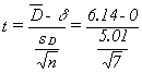
As is usual in this kind of situation, LaTonya is hoping that the data support Ha, but she wants to be confident that it does before she decides her workers are earning above average wages. Remember that she will compute a t-score for her sample using $11.71 for μ. If her t-score is negative or close to zero, she will conclude that the data support Ho. Only if her t-score is large and positive will she go with Ha. She decides to use α=.025 because she is unwilling to take much risk of saying the workers earn above average wages when they really do not. Because her sample has n=7, she has 6 df. Looking at the table, she sees that the data will support Ha, the workers earn more than average, only if the sample t-score is greater than 2.447.
Finding the sample mean and standard deviation, x = $10.83 and s = $.749, LaTonya computes her sample t-score:
[latex]t=(\bar{x}-\mu)/(s/\sqrt{n})=(10.83-11.71)/(.749/\sqrt{7})=1.48[/latex]
Because her sample t is not greater than +2.447, the H0 is not rejected, indicating that LaTonya concludes that she will have to raise the piece rates EDC pays in order to be really sure that mean hourly earnings are above the local average wage.
If LaTonya had simply wanted to know if EDC’s workers earned the same as other workers in the area, she would have used a two-tail test. In that case, her hypotheses would have been:
[latex]H_o: \mu = \$11.71\;and\;H_a: \mu \neq \$11.71[/latex]
Using α=.10, LaTonya would split the .10 between the two tails since the data support Ha if the sample t-score is either large and negative or large and positive. Her arithmetic is the same, her sample t-score is still 1.41, but she now will decide that the data support Ha only if it is outside ±1.943. In this case, LaTonya will again reject H0, and conclude that the EDC’s workers do not earn the same as other workers in the area.
An alternative to choosing an alpha
Many researchers now report how unusual the sample t-score would be if the null hypothesis were true rather than choosing an α and stating whether the sample t-score implies the data support one or the other of the hypotheses based on that α. When a researcher does this, he is essentially letting the reader of his report decide how much risk to take of making which kind of mistake. There are even two ways to do this. If you look at a portion of any textbook t-table, you will see that it is not set up very well for this purpose; if you wanted to be able to find out what part of a t-distribution was above any t-score, you would need a table that listed many more t-scores. Since the t-distribution varies as the df. changes, you would really need a whole series of t-tables, one for each df. Fortunately, the interactive Excel template provided in Figure 5.1 will enable you to have a complete picture of the t-table and its distribution.
The old-fashioned way of making the reader decide how much of which risk to take is to not state an α in the body of your report, but only give the sample t-score in the main text. To give the reader some guidance, you look at the usual t-table and find the smallest α, say it is .01, that has a t-value less than the one you computed for the sample. Then write a footnote saying, “The data support the alternative hypothesis for any α > .01.”
The more modern way uses the capability of a computer to store lots of data. Many statistical software packages store a set of detailed t-tables, and when a t-score is computed, the package has the computer look up exactly what proportion of samples would have t-scores larger than the one for your sample. Table 5.2 shows the computer output for LaTonya’s problem from a typical statistical package. Notice that the program gets the same t-score that LaTonya did, it just goes to more decimal places. Also notice that it shows something called the p-value. The p-value is the proportion of t-scores that are larger than the one just computed. Looking at the example, the computed t statistic is 1.48 and the p-value is .094. This means that if there are 6 df, a little more than 9 per cent of samples will have a t-score greater than 1.48. Remember that LaTonya used an α = .025 and decided that the data supported Ho, the p-value of .094 means that Ho, would be supported for any α less than .094. Since LaTonya had used α = .025, this p-value means she does not find support for Ho.
| Hypothesis test: Mean |
| Null hypothesis: Mean = $11.71 |
| Alternative: greater than |
| Computed t statistic = 1.48 |
| p-value = .094 |
The p-value approach is becoming the preferred way to present research results to audiences of professional researchers. Most of the statistical research conducted for a business firm will be used directly for decision making or presented to an audience of executives to aid them in making a decision. These audiences will generally not be interested in deciding for themselves which hypothesis the data support. When you are making a presentation of results to your boss, you will want to simply state which hypothesis the evidence supports. You may decide by using either the traditional α approach or the more modern p– value approach, but deciding what the evidence says is probably your job.
Another t-test: do these two (independent) samples come from populations with the same mean?
One of the other statistics that has a sampling distribution that follows the t-distribution is the difference between two sample means. If samples of one size (n1) are taken from one normal population and samples of another size (n2) are taken from another normal population (and the populations have the same standard deviation), then a statistic based on the difference between the sample means and the difference between the population means is distributed like t with n1 + n2 – 2 degrees of freedom. These samples are independent because the members in one sample do not affect which members are in the other sample. You can choose the samples independently of each other, and the two samples do not need to be the same size. The t-statistic is:
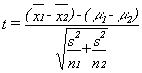
where
xi = the mean of sample i
μi = the mean of population i
s2 = the pooled variance
ni = the size of sample i
The usual case is to test to see if the samples come from populations with the same mean, the case where (μ1 – μ2) = 0. The pooled variance is simply a weighted average of the two sample variances, with the weights based on the sample sizes. This means that you will have to calculate the pooled variance before you calculate the t-score. The formula for pooled variance is:
![]()
To use the pooled variance t-score, it is necessary to assume that the two populations have equal variances. If you are wondering about why statisticians make a strong assumption in order to use such a complicated formula, it is because the formula that does not need the assumption of equal variances is even more complicated, and reduces the degrees of freedom in the final statistic. In any case, unless you have small samples, the amount of arithmetic needed means that you will probably want to use a statistical software package for this test. You should also note that you can test to see if two samples come from populations that are any hypothesized distance apart by setting (μ1 – μ2) equal to that distance.
In a report published in a 2001 issue of University Affairs,[1] Frank claimed that researchers found a drop in the number of students getting low grades in most courses, and an increase in the number getting high grades (Frank, 2001). This issue is also known as grade inflation. Nora Alston chairs the Economics Department at Oaks College, and the Dean has sent her a copy of the report with a note attached saying, “Is this true here at Oaks? Let me know.” Dr. Alston is not sure if the Dean would be happier if economics grades were higher or lower than other grades, but the report claims that economics grades are lower. Her first stop is the Registrar’s office.
She has the clerk in that office pick a sample of 10 class grade reports from across the college spread over the past three semesters. She also has the clerk pick out a sample of 10 reports for economics classes. She ends up with a total of 38 grades for economics classes and 51 grades for other classes. Her hypotheses are:
[latex]H_o: \mu_{econ} - \mu_{other} \geq 0[/latex]
[latex]H_a: \mu_{econ} - \mu_{other} < 0[/latex] She decides to use α = .05$ .
This is a lot of data, and Dr. Alston knows she will want to use the computer to help. She initially thought she would use a spreadsheet to find the sample means and variances, but after thinking a minute, she decided to use a statistical software package. The one she is most familiar with is called SAS. She loads SAS onto her computer, enters the data, and gives the proper SAS commands. The computer gives her the output shown in Table 5.3.
| Table 5.3 The SAS System Software Output for Dr. Alston’s Grade Study | ||||||
| TTFST Procedure | ||||||
| Variable: GRADE | ||||||
| Dept | N | Mean | Dev | Std Error | Minimum | Maximum |
| Econ | 38 | 2.28947 | 1.01096 | .16400 | 0 | 4.00000 |
| Variance | t | df | Prob>[t] |
| Unequal | -2.3858 | 85.1 | .0193 |
| Equal | -2.3345 | 87.0 | .0219 |
| For Ho: Variances are equal, f=1.35, df[58.37], Prob>f=.3485 | |||
Dr. Alston has 87 df, and has decided to use a one-tailed, left tail test with α = .05$. She goes to her t-table and finds that 87 df does not appear, the table skipping from 60 to 120 df. There are two things she could do. She could try to interpolate the t-score that leaves .05 in the tail with 87 df, or she could choose between the t-value for 60 and 120 in a conservative manner. Using the conservative choice is the best initial approach, and looking at her table she sees that for 60 df .05 of t-scores are less than -1.671,and for 120 df, .05 are less than -1.658. She does not want to conclude that the data support economics grades being lower unless her sample t-score is far from zero, so she decides that she will accept Ha if her sample t is to the left of -1.671. If her sample t happens to be between -1.658 and -1.671, she will have to interpolate.
Looking at the SAS output, Dr. Alston sees that her t-score for the equal variances formula is -2.3858, which is well below -1.671. She concludes that she will tell the Dean that economics grades are lower than grades elsewhere at Oaks College.
Notice that SAS also provides the t-score and df for the case where equal variances are not assumed in the unequal line. SAS also provides a p-value, but it is for a two-tail test because it gives the probability that a t with a larger absolute value, >|T|, occurs. Be careful when using the p-values from software: notice if they are one-tail or two-tail p-values before you make your report.
A third t-test: do these (paired) samples come from the sample population?
Managers are often interested in before and after questions. As a manager or researcher, you will often want to look at longitudinal studies, studies that ask about what has happened to an individual as a result of some treatment or across time. Are they different after than they were before? For example, if your firm has conducted a training program, you will want to know if the workers who participated became more productive. If the work area has been rearranged, do workers produce more than before? Though you can use the difference of means test developed earlier, this is a different situation. Earlier, you had two samples that were chosen independently of each other; you might have a sample of workers who received the training and a sample of workers who had not. The situation for this test is different; now you have a sample of workers, and for each worker, you have measured their productivity before the training or rearrangement of the work space, and you have measured their productivity after. For each worker, you have a pair of measures, before and after. Another way to look at this is that for each member of the sample you have a difference between before and after.
You can test to see if these differences equal zero, or any other value, because a statistic based on these differences follows the t-distribution for n-1 df when you have n matched pairs. That statistic is:

where
D = the mean of the differences in the pairs in the sample
δ = the mean of the differences in the pairs in the population
sD = the standard deviation of the differences in the sample
n = the number of pairs in the sample
It is a good idea to take a minute and figure out this formula. There are paired samples, and the differences in those pairs, the D’s, are actually a population. The mean of those D’s is δ. Any sample of pairs will also yield a sample of D’s. If those D’s are normally distributed, then the t-statistic in the formula above will follow the t-distribution. If you think of the D’s as being the same as x’s in the t-formula at the beginning of the chapter, and think of δ as the population mean, you should realize that this formula is really just that basic t formula.
Lew Podolsky is division manager for Dairyland Lighting, a manufacturer of outdoor lights for parking lots, barnyards, and playing fields. Dairyland Lighting organizes its production work by teams. The size of the team varies somewhat with the product being assembled, but there are usually three to six in a team, and a team usually stays together for a few weeks assembling the same product. Dairyland Lighting has two new plants: one in Oshawa, Ontario, and another in Osoyoos, British Columbia, that serves their Canadian west coast customers. Lew has noticed that productivity seems to be lower in Osoyoos during the summer, a problem that does not occur at their plant in Oshawa. After visiting the Osoyoos plant in July, August, and November, and talking with the workers during each visit, Lew suspects that the un-air-conditioned plant just gets too hot for good productivity. Unfortunately, it is difficult to directly compare plant-wide productivity at different times of the year because there is quite a bit of variation in the number of employees and the product mix through the year. Lew decides to see if the same workers working on the same products are more productive on cool days than hot days by asking the local manager, Dave Mueller, to find a cool day and a hot day from the previous fall and choose ten work teams who were assembling the same products on the two days. Dave sends Lew the data found in Table 5.4.
| Team leader | Output—cool day | Output—hot day | Difference (cool-hot) |
|---|---|---|---|
| November 14 | July 20 | ||
| Martinez | 153 | 149 | 4 |
| McAlan | 167 | 170 | -3 |
| Wilson | 164 | 155 | 9 |
| Burningtree | 183 | 179 | 4 |
| Sanchez | 177 | 167 | 10 |
| Lilly | 162 | 150 | 12 |
| Cantu | 165 | 158 | 7 |
Lew decides that if the data support productivity being higher on cool days, he will call in a heating/air-conditioning contractor to get some cost estimates so that he can decide if installing air conditioning in the Osoyoos plant is cost effective. Notice that he has matched pairs data — for each team he has production on November 14, a cool day, and on July 20, a hot day. His hypotheses are:
[latex]H_o: \delta \leq 0\;and\;H_a: \delta > 0[/latex]
Using α = .05 in this one-tail test, Lew will decide to call the engineer if his sample t-score is greater than 1.943, since there are 6 df. Using the interactive Excel template in Figure 5.2, Lew finds:
![]()
![]()
and his sample t-score is
and
![]()
Figure 5.2 Interactive Excel Template for Paired t-Test - see Appendix 5.
All these calculations can also be done in the interactive Excel template in Figure 5.2. You can add the two columns of data for cool and hot days and set your α level. The associated t-distribution will automatically adjust based on your data and the selected level of α. You can also see the p-value in the dark blue, and the selected α in the red-shaded areas on this graph. Because his sample t-score is greater than 1.943, or the p-value is less than the alpha, Lew gets out the telephone book and looks under air conditioning contractors to call for some estimates.
Summary
The t-tests are commonly used hypothesis tests. Researchers often find themselves in situations where they need to test to see if a sample comes from a certain population, and therefore test to see if the sample probably came from a population with that certain mean. Even more often, researchers will find themselves with two samples and want to know if the samples come from the same population, and will test to see if the samples probably come from populations with the same mean. Researchers also frequently find themselves asking if two sets of paired samples have equal means. In any case, the basic strategy is the same as for any hypothesis test. First, translate the question into null and alternative hypotheses, making sure that the null hypothesis includes an equal sign. Second, choose α. Third, compute the relevant statistics, here the t-score, from the sample or samples. Fourth, using the tables, decide if the sample statistic leads you to conclude that the sample came from a population where the null hypothesis is true or a population where the alternative is true.
The t-distribution is also used in testing hypotheses in other situations since there are other sampling distributions with the same t-distribution shape. So, remember how to use the t-tables for later chapters.
Statisticians have also found how to test to see if three or more samples come from populations with the same mean. That technique is known as one-way analysis of variance. The approach used in analysis of variance is quite different from that used in the t-test. It will be covered in Chapter 6.
Chapter 6. F-Test and One-Way ANOVA
F-distribution
Years ago, statisticians discovered that when pairs of samples are taken from a normal population, the ratios of the variances of the samples in each pair will always follow the same distribution. Not surprisingly, over the intervening years, statisticians have found that the ratio of sample variances collected in a number of different ways follow this same distribution, the F-distribution. Because we know that sampling distributions of the ratio of variances follow a known distribution, we can conduct hypothesis tests using the ratio of variances.
The F-statistic is simply:
[latex]F = s^2_1 / s^2_2[/latex]
where s12 is the variance of sample 1. Remember that the sample variance is:
[latex]s^2 = \sum(x - \overline{x})^2 / (n-1)[/latex]
Think about the shape that the F-distribution will have. If s12 and s22 come from samples from the same population, then if many pairs of samples were taken and F-scores computed, most of those F-scores would be close to one. All of the F-scores will be positive since variances are always positive — the numerator in the formula is the sum of squares, so it will be positive, the denominator is the sample size minus one, which will also be positive. Thinking about ratios requires some care. If s12 is a lot larger than s22, F can be quite large. It is equally possible for s22 to be a lot larger than s12, and then F would be very close to zero. Since F goes from zero to very large, with most of the values around one, it is obviously not symmetric; there is a long tail to the right, and a steep descent to zero on the left.
There are two uses of the F-distribution that will be discussed in this chapter. The first is a very simple test to see if two samples come from populations with the same variance. The second is one-way analysis of variance (ANOVA), which uses the F-distribution to test to see if three or more samples come from populations with the same mean.
A simple test: Do these two samples come from populations with the same variance?
Because the F-distribution is generated by drawing two samples from the same normal population, it can be used to test the hypothesis that two samples come from populations with the same variance. You would have two samples (one of size n1 and one of size n2) and the sample variance from each. Obviously, if the two variances are very close to being equal the two samples could easily have come from populations with equal variances. Because the F-statistic is the ratio of two sample variances, when the two sample variances are close to equal, the F-score is close to one. If you compute the F-score, and it is close to one, you accept your hypothesis that the samples come from populations with the same variance.
This is the basic method of the F-test. Hypothesize that the samples come from populations with the same variance. Compute the F-score by finding the ratio of the sample variances. If the F-score is close to one, conclude that your hypothesis is correct and that the samples do come from populations with equal variances. If the F-score is far from one, then conclude that the populations probably have different variances.
The basic method must be fleshed out with some details if you are going to use this test at work. There are two sets of details: first, formally writing hypotheses, and second, using the F-distribution tables so that you can tell if your F-score is close to one or not. Formally, two hypotheses are needed for completeness. The first is the null hypothesis that there is no difference (hence null). It is usually denoted as Ho. The second is that there is a difference, and it is called the alternative, and is denoted H1 or Ha.
Using the F-tables to decide how close to one is close enough to accept the null hypothesis (truly formal statisticians would say "fail to reject the null") is fairly tricky because the F-distribution tables are fairly tricky. Before using the tables, the researcher must decide how much chance he or she is willing to take that the null will be rejected when it is really true. The usual choice is 5 per cent, or as statisticians say, "α - .05". If more or less chance is wanted, α can be varied. Choose your α and go to the F-tables. First notice that there are a number of F-tables, one for each of several different levels of α (or at least a table for each two α’s with the F-values for one α in bold type and the values for the other in regular type). There are rows and columns on each F-table, and both are for degrees of freedom. Because two separate samples are taken to compute an F-score and the samples do not have to be the same size, there are two separate degrees of freedom — one for each sample. For each sample, the number of degrees of freedom is n-1, one less than the sample size. Going to the table, how do you decide which sample’s degrees of freedom (df) are for the row and which are for the column? While you could put either one in either place, you can save yourself a step if you put the sample with the larger variance (not necessarily the larger sample) in the numerator, and then that sample’s df determines the column and the other sample’s df determines the row. The reason that this saves you a step is that the tables only show the values of F that leave α in the right tail where F > 1, the picture at the top of most F-tables shows that. Finding the critical F-value for left tails requires another step, which is outlined in the interactive Excel template in Figure 6.1. Simply change the numerator and the denominator degrees of freedom, and the α in the right tail of the F-distribution in the yellow cells.
Figure 6.1 Interactive Excel Template of an F-Table - see Appendix 6.
F-tables are virtually always printed as one-tail tables, showing the critical F-value that separates the right tail from the rest of the distribution. In most statistical applications of the F-distribution, only the right tail is of interest, because most applications are testing to see if the variance from a certain source is greater than the variance from another source, so the researcher is interested in finding if the F-score is greater than one. In the test of equal variances, the researcher is interested in finding out if the F-score is close to one, so that either a large F-score or a small F-score would lead the researcher to conclude that the variances are not equal. Because the critical F-value that separates the left tail from the rest of the distribution is not printed, and not simply the negative of the printed value, researchers often simply divide the larger sample variance by the smaller sample variance, and use the printed tables to see if the quotient is "larger than one", effectively rigging the test into a one-tail format. For purists, and occasional instances, the left-tail critical value can be computed fairly easily.
The left-tail critical value for x, y degrees of freedom (df) is simply the inverse of the right-tail (table) critical value for y, x df. Looking at an F-table, you would see that the F-value that leaves α - .05 in the right tail when there are 10, 20 df is F=2.35. To find the F-value that leaves α - .05 in the left tail with 10, 20 df, look up F=2.77 for α - .05, 20, 10 df. Divide one by 2.77, finding .36. That means that 5 per cent of the F-distribution for 10, 20 df is below the critical value of .36, and 5 per cent is above the critical value of 2.35.
Putting all of this together, here is how to conduct the test to see if two samples come from populations with the same variance. First, collect two samples and compute the sample variance of each, s12 and s22. Second, write your hypotheses and choose α . Third find the F-score from your samples, dividing the larger s2 by the smaller so that F>1. Fourth, go to the tables, find the table for α/2, and find the critical (table) F-score for the proper degrees of freedom (n-1 and n-1). Compare it to the samples’ F-score. If the samples’ F is larger than the critical F, the samples’ F is not "close to one", and Ha the population variances are not equal, is the best hypothesis. If the samples’ F is less than the critical F, Ho, that the population variances are equal, should be accepted.
Example #1
Lin Xiang, a young banker, has moved from Saskatoon, Saskatchewan, to Winnipeg, Manitoba, where she has recently been promoted and made the manager of City Bank, a newly established bank in Winnipeg with branches across the Prairies. After a few weeks, she has discovered that maintaining the correct number of tellers seems to be more difficult than it was when she was a branch assistant manager in Saskatoon. Some days, the lines are very long, but on other days, the tellers seem to have little to do. She wonders if the number of customers at her new branch is simply more variable than the number of customers at the branch where she used to work. Because tellers work for a whole day or half a day (morning or afternoon), she collects the following data on the number of transactions in a half day from her branch and the branch where she used to work:
Winnipeg branch: 156, 278, 134, 202, 236, 198, 187, 199, 143, 165, 223
Saskatoon branch: 345, 332, 309, 367, 388, 312, 355, 363, 381
She hypothesizes:
[latex]H_o: \sigma^2_W = \sigma^2_S[/latex]
[latex]H_a: \sigma^2_W \neq \sigma^2_S[/latex]
She decides to use α - .05. She computes the sample variances and finds:
[latex]s^2_W =1828.56[/latex]
[latex]s^2_S =795.19[/latex]
Following the rule to put the larger variance in the numerator, so that she saves a step, she finds:
[latex]F = s^2_W/s^2_S = 1828.56/795.19 = 2.30[/latex]
Figure 6.2 Interactive Excel Template for F-Test - see Appendix 6.
Using the interactive Excel template in Figure 6.2 (and remembering to use the α - .025 table because the table is one-tail and the test is two-tail), she finds that the critical F for 10,8 df is 4.30. Because her F-calculated score from Figure 6.2 is less than the critical score, she concludes that her F-score is "close to one", and that the variance of customers in her office is the same as it was in the old office. She will need to look further to solve her staffing problem.
Analysis of variance (ANOVA)
The importance of ANOVA
A more important use of the F-distribution is in analyzing variance to see if three or more samples come from populations with equal means. This is an important statistical test, not so much because it is frequently used, but because it is a bridge between univariate statistics and multivariate statistics and because the strategy it uses is one that is used in many multivariate tests and procedures.
One-way ANOVA: Do these three (or more) samples all come from populations with the same mean?
This seems wrong — we will test a hypothesis about means by analyzing variance. It is not wrong, but rather a really clever insight that some statistician had years ago. This idea — looking at variance to find out about differences in means — is the basis for much of the multivariate statistics used by researchers today. The ideas behind ANOVA are used when we look for relationships between two or more variables, the big reason we use multivariate statistics.
Testing to see if three or more samples come from populations with the same mean can often be a sort of multivariate exercise. If the three samples came from three different factories or were subject to different treatments, we are effectively seeing if there is a difference in the results because of different factories or treatments — is there a relationship between factory (or treatment) and the outcome?
Think about three samples. A group of x’s have been collected, and for some good reason (other than their x value) they can be divided into three groups. You have some x’s from group (sample) 1, some from group (sample) 2, and some from group (sample) 3. If the samples were combined, you could compute a grand mean and a total variance around that grand mean. You could also find the mean and (sample) variance within each of the groups. Finally, you could take the three sample means, and find the variance between them. ANOVA is based on analyzing where the total variance comes from. If you picked one x, the source of its variance, its distance from the grand mean, would have two parts: (1) how far it is from the mean of its sample, and (2) how far its sample’s mean is from the grand mean. If the three samples really do come from populations with different means, then for most of the x’s, the distance between the sample mean and the grand mean will probably be greater than the distance between the x and its group mean. When these distances are gathered together and turned into variances, you can see that if the population means are different, the variance between the sample means is likely to be greater than the variance within the samples.
By this point in the book, it should not surprise you to learn that statisticians have found that if three or more samples are taken from a normal population, and the variance between the samples is divided by the variance within the samples, a sampling distribution formed by doing that over and over will have a known shape. In this case, it will be distributed like F with m-1, n-m df, where m is the number of samples and n is the size of the m samples altogether. Variance between is found by:
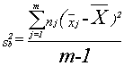
where xj is the mean of sample j, and x is the grand mean.
The numerator of the variance between is the sum of the squares of the distance between each x’s sample mean and the grand mean. It is simply a summing of one of those sources of variance across all of the observations.
The variance within is found by:
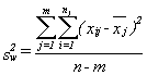
Double sums need to be handled with care. First (operating on the inside or second sum sign) find the mean of each sample and the sum of the squares of the distances of each x in the sample from its mean. Second (operating on the outside sum sign), add together the results from each of the samples.
The strategy for conducting a one-way analysis of variance is simple. Gather m samples. Compute the variance between the samples, the variance within the samples, and the ratio of between to within, yielding the F-score. If the F-score is less than one, or not much greater than one, the variance between the samples is no greater than the variance within the samples and the samples probably come from populations with the same mean. If the F-score is much greater than one, the variance between is probably the source of most of the variance in the total sample, and the samples probably come from populations with different means.
The details of conducting a one-way ANOVA fall into three categories: (1) writing hypotheses, (2) keeping the calculations organized, and (3) using the F-tables. The null hypothesis is that all of the population means are equal, and the alternative is that not all of the means are equal. Quite often, though two hypotheses are really needed for completeness, only Ho is written:
[latex]H_o: m_1=m_2=\ldots=m_m[/latex]
Keeping the calculations organized is important when you are finding the variance within. Remember that the variance within is found by squaring, and then summing, the distance between each observation and the mean of its sample. Though different people do the calculations differently, I find the best way to keep it all straight is to find the sample means, find the squared distances in each of the samples, and then add those together. It is also important to keep the calculations organized in the final computing of the F-score. If you remember that the goal is to see if the variance between is large, then its easy to remember to divide variance between by variance within.
Using the F-tables is the third detail. Remember that F-tables are one-tail tables and that ANOVA is a one-tail test. Though the null hypothesis is that all of the means are equal, you are testing that hypothesis by seeing if the variance between is less than or equal to the variance within. The number of degrees of freedom is m-1, n-m, where m is the number of samples and n is the total size of all the samples together.
Example #2
The young bank manager in Example 1 is still struggling with finding the best way to staff her branch. She knows that she needs to have more tellers on Fridays than on other days, but she is trying to find if the need for tellers is constant across the rest of the week. She collects data for the number of transactions each day for two months. Here are her data:
Mondays: 276, 323, 298, 256, 277, 309, 312, 265, 311
Tuesdays: 243, 279, 301, 285, 274, 243, 228, 298, 255
Wednesdays: 288, 292, 310, 267, 243, 293, 255, 273
Thursdays: 254, 279, 241, 227, 278, 276, 256, 262
She tests the null hypothesis:
[latex]H_o: m_m=m_{tu}=m_w=m_{th}[/latex]
and decides to use α - .05. She finds:
m = 291.8
tu = 267.3
w = 277.6
th = 259.1
and the grand mean = 274.3
She computes variance within:
[(276-291.8)2+(323-291.8)2+...+(243-267.6)2+...+(288-277.6)2+...+(254-259.1)2]/[34-4]=15887.6/30=529.6
Then she computes variance between:
[9(291.8-274.3)2+9(267.3-274.3)2+8(277.6-274.3)2+8(259.1-274.3)2]/[4-1]
= 5151.8/3 = 1717.3
She computes her F-score:
![]()
Figure 6.3 Interactive Excel Template for One-Way ANOVA - see Appendix 6.
You can enter the number of transactions each day in the yellow cells in Figure 6.3, and select the α. As you can then see in Figure 6.3, the calculated F-value is 3.24, while the F-table (F-Critical) for α - .05 and 3, 30 df, is 2.92. Because her F-score is larger than the critical F-value, or alternatively since the p-value (0.036) is less than α - .05, she concludes that the mean number of transactions is not equal on different days of the week, or at least there is one day that is different from others. She will want to adjust her staffing so that she has more tellers on some days than on others.
Summary
The F-distribution is the sampling distribution of the ratio of the variances of two samples drawn from a normal population. It is used directly to test to see if two samples come from populations with the same variance. Though you will occasionally see it used to test equality of variances, the more important use is in analysis of variance (ANOVA). ANOVA, at least in its simplest form as presented in this chapter, is used to test to see if three or more samples come from populations with the same mean. By testing to see if the variance of the observations comes more from the variation of each observation from the mean of its sample or from the variation of the means of the samples from the grand mean, ANOVA tests to see if the samples come from populations with equal means or not.
ANOVA has more elegant forms that appear in later chapters. It forms the basis for regression analysis, a statistical technique that has many business applications; it is covered in later chapters. The F-tables are also used in testing hypotheses about regression results.
This is also the beginning of multivariate statistics. Notice that in the one-way ANOVA, each observation is for two variables: the x variable and the group of which the observation is a part. In later chapters, observations will have two, three, or more variables.
The F-test for equality of variances is sometimes used before using the t-test for equality of means because the t-test, at least in the form presented in this text, requires that the samples come from populations with equal variances. You will see it used along with t-tests when the stakes are high or the researcher is a little compulsive.
- Frank, T. (2001, February). New study says grades are inflated at Ontario universities. University Affairs, 29. ↵
